Low-level disk storage
This article is about how information is stored on a floppy disk on a fairly low level. From a MSX background perspective.
I’m going to assume that you, the reader, already have some basic knowledge. Here’s a refresher:
- A floppy disk is a nearly square plastic enclosure around a circular disk. This disk is made from a material that can be magnetized.
- Either a single or both sides of this disk can be used to store information.
- Floppy disks are used in a disk-drive. This drive contains a read/write-head to retrieve or modify the information stored on the disk. More specifically reading involves sensing the patterns in the magnetization of the disk. Writing means modifying those patterns.
- The disk can rotate. While it rotates, the drive-head enscribes a circle on the surface of the disk. Such a circle is called a track.
- The drive-head can move radially across the disk, into discrete positions. Each such position gives rise to a different track. Typically there are 80 different tracks (on each side of the disk).
- Each track is further subdivided into sectors. Typically 9 sectors per track.
In this article we’ll go a few steps further:
- We’ll see that sectors are split into a header- and a data-block.
- There are various gaps between these block. We’ll see why these gaps are needed.
- These blocks store information as bytes, 8 bits per byte. We’ll see how these bits are actually stored as magnetic patterns on the disk surface. We’ll see that bits still have a sub-structure.
This article is not about low level disk programming:
- We’ll not talk about using the BDOS to read/write a disk.
- We’ll not talk about the interpretation of the data stored on the disk. So we’ll not talk about stuff like the boot-sector, the FAT-filesystem, ...
- We’ll not talk about how to directly access the floppy disk controller (FDC). Though this article does contain useful background information for that purpose.
Chapter one focusses on how bits are stored (in a track) on the disk.
In chapter two we’ll see that grouping 8 bits into a byte is not as trivial as you may think.
Chapter three explores what formatting a track means. That is: how the bytes from the previous chapter are interpreted to form a track-layout.
In chapter four we look at the disk from a FDC-point of view. We won’t talk about programming the FDC, instead we’ll explore how the FDC interprets and modifies the information on the disk.
Focus on one specific disk type
There are many different types of floppy disks. But this article assumes a MSX background, and therefor we’ll mostly focus on one specific disk type:
- 3.5 inch, double density (DD), double sided (DS), 80 tracks per side.
- We’ll mostly assume a normally formatted disk with 9 sectors per track. Occasionally we’ll mention deviations, but copy-protected disks are mostly outside the scope of this article.
Here’s an image of such a disk.
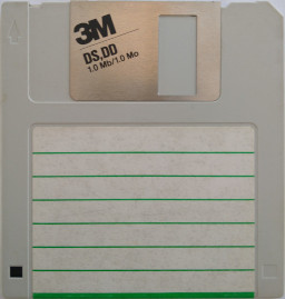
Notice how it’s labeled with “1.0 Mb” (detail: “1.0 MB” would be more correct, as it’s really 1 MegaByte, not 1 MegaBit). Although these disks were often advertised as holding 1MB of information, in practice they can only store 720kB. Is this false advertising? Let’s examine what’s going on.
These disks rotate at 300rpm (=300/60 = 5 rotations per second). And for double-density disks, the data-rate is 250k bits per second. So per track that means:
- 250k bits per second / 5 rotations per second
- = 50k bits per rotation / 8 bits per byte
- = 6250 bytes per track
For the full disk that then is:
- 6250 bytes per track * 80 tracks per side * 2 sides per disk
- = 1000000 bytes per disk
And 1 million bytes is marketing-speak for 1MB (a full MegaByte is actually 1048576 bytes). So although the above is technically correct, you also see disks that are more honestly labeled as:
- 1.0MB (unformatted)
- 720kB (formatted)
In chapter three we’ll see what exactly this ‘formatting’ means. Why it takes so much space away. And why it’s needed.
Although this article focuses on this one specific disk type, most of the information is type-agnostic. Or else it can easily be generalized or extrapolated to other types.
Table of contents
- Introduction
- Table of contents
- 1. How are bits stored as magnetic patterns
- 2. From bit-stream to byte-stream
- 3. Track layout
- 4. Floppy disk controller (FDC)
- Appendix A: CRC calculation for “CRC-16-CCITT”
1. How are bits stored as magnetic patterns
In the introduction we talked about high level concepts like tracks and sectors. In this section we go to the other end of the spectrum: How are bits represented on disk. We’ll see that bits are even further subdivided into smaller units.
1.1. Naive solution
You probably know that floppy disks store information on a magnetic material. More specifically this material can be magnetically oriented in one of two different directions. I actually don’t know how these directions are physically oriented:
- It could be orthogonal on the surface of the disk (in-to or out-from the disk surface).
- It could be along the disk surface, directed radially towards inner/outer tracks (towards the center or towards the perimeter).
- Or it could be along the disk surface, tangential to the direction of the track (forward or backward along the direction of the track).
But, for this article, that’s not important. It only matters that there are two different directions. For simplicity let’s just call these directions “up” and “down”.
At first sight it may seem that these two orientations can directly be used to store bits: store a 0-bit as “up” and a 1-bit as “down”. For example the 2-byte sequence 0x48, 0x0B could then be stored like this:
Why this doesn’t work
Reason 1: clock synchronization
A disk can be written in one disk drive, and then later be read in another disk drive. And obviously we want to read the same data from the second drive as was written by the first drive.
But disk drives have manufacturing tolerances, including the exact rotation speed of the drive. For example one drive might rotate at 295rpm while another rotates at 305rpm, instead of both at the exact nominal 300rpm.
Also the clock that drives the data-rate, nominally 250k bits/s, might be slightly different between the two systems.
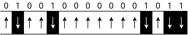
More in detail: while the disk is rotating, at every tick of the clock, the drive would sample the magnetic orientation of the material under the read-head. One orientation means a 0-bit, the other orientation means a 1-bit. But this approach causes problems when the rotation-speed and/or the sample-rate is not exactly the same between the time the disk was written and when it is read again. This is especially true when there are long stretches of consecutive 0- or 1-bits. You can intuitively see this in the following diagram:

Without peeking at the previous diagram, can you tell how long the large (white) middle region is? ... Ok, you can peek now: there were 7 consecutive 0-bits. This becomes even harder for longer stretches of identical bits. And in facts these stretches can become arbitrarily long. Also the rotation speed can vary, and along with it the length, or duration, of these stretches. And then it becomes impossible to correctly recover the original bit-stream.
More technically this problem is called “clock recovery”. If somehow we could recover the clock signal (synchronized to the rotation of the disk) used during writing of the disk, then we can use that clock as the reference, and correctly retrieve the original information.
This naive solution doesn’t work, it does not contain enough information to also recover the clock. To fix this we’ll have to ensure there are never too long stretches (=regions on the disk) without changes in magnetic orientation. We’ll see how to achieve this in the later sub-sections about encodings.
Reason 2: changing vs absolute magnetic orientation
But first we’ll look at a second problem. It’s related to how the disk drive’s read-head is constructed.
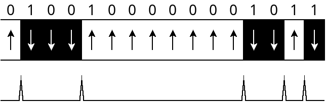
Basically the read-head contains a copper coil. The surfaces of the floppy disk, which has regions with different magnetic orientations, is rotating in close proximity to this coil. From physics lessons you may remember that a changing magnetic field induces an electric current in a electrically conducting wire (=coil). In a diagram this looks as follows:

Compare this to the previous diagrams: notice how for every switch from black-to-white or from white-to-black there is a pulse.
So the disk drive only sees these pulses. All it can do is time the duration between these pulses, and all information should be reconstructed from these measured durations.
An important detail is that the drive sees the same pulse for a change from up-to-down than for down-to-up. In other words: the drive can only measure “changes in magnetic orientation” (we’ll call these “flux-reversals”), but it can not measure the absolute orientation of the magnetic field (up or down).
I’m guessing a bit in this paragraph: in principle the drive could retrieve the orientation of the magnetic field by looking at the direction of the induced current: it will be opposite for changes from up-to-down than for changes from down-to-up. Though as far as I understand the disk drive does not use that extra information (maybe it’s cheaper to manufacture that way??). So really the drive only sees flux-reversals, but no absolute magnetic orientation.
With this complication in mind, the above example becomes ambiguous. The sequence can either be interpreted as “0100100000001011” or as “1011011111110100”. That is: all 0- and 1-bits flipped.
Luckily this problem is easy to fix: instead of directly encoding 0- and 1-bit as up/down magnetic orientations, we instead encode:
- a 0-bit as NO change in the magnetic orientation (NO flux-reversal)
- a 1-bit as A change in the magnetic orientation (A flux-reversal)
The above example, store the byte-sequence 0x48 0x0B, then becomes:
At the hardware level, decoding this signal is very simple:
- When the read-head measures NO pulse: output a 0-bit.
- When the read-head measures A pulse: output a 1-bit.
But of course long stretches without any pulses (no flux-reversals) remain a problem.
Intermezzo: clock-recovery via a phase-locked-loop (PLL)
Suppose that we can somehow guarantee there are sufficient flux-reversals. We’ll see how to achieve that in the next two sub-sections. For example suppose the expected duration between two pulses is either 4ms, 8ms or 12ms. At 250k bits/s that means 0, 1 or 2 (but no more) 0-bits between two every two 1-bits. But because of variations in rotation speed we may not always measure exactly 4ms, 8ms or 12ms.
Some easy examples. Suppose we measure:
- 4.1ms: that’s likely supposed to be 4ms, so 2 consecutive 1-bits.
- 7.8ms: also easy, this was likely 8ms, so the bit-pattern “101”.
Now some more difficult scenarios. Not needed to understand these in detail. Suppose we measure something close to the halfway-point between two expected values:
- If (only) the previous pulse came a bit sooner than expected, this could be a local defect. In other words: a single pulse that’s a bit out-of-place. Then we can reasonably expect that the next pulse will arrive a bit later (to compensate). And then we’re better off to round close-to-the-halfway-point measurements down.
- On the other hand it’s possible that not only the last (single) pulse, but a whole lot of earlier pulses all arrived sooner than expected. In that case the more likely interpretation is that the disk is spinning too fast. And then it’s better to round close-to-halfway measurements up instead of down.
- And there are many other scenarios ...
But again the details aren’t important. I only wanted to demonstrate this is a non-trivial problem. But it is a problem with a well known solution:
A “Phase Locked Loop” (PLL) is a circuit that:
- Looks at the recent history of the signal. In our case: the duration between pulses.
- From this it learns the base-duration between possible pulses. That is: if we see a pulse now, we expect to see another pulse either 4, 8 or 12ms later. So every 4ms there possibly is a pulse. In other words: it learns the underlying clock frequency that generates the pulses.
- It also learns the expected moments in time when a pulse can be expected. In other words: it learns the phase of the generating-clock.
- This works better if the ratio between the longest and the shortest expected duration is not too large. In this example: that ratio is 12ms / 4ms = 3.
- It also works better if the measured clock does not deviate too much from the original clock. In this case that means: the rotation speed difference between writing and reading is not too large.
To summarize: after some training, a PLL can recover the original clock from a signal, both the frequency and the phase. That’s what we called “clock-recovery” in the previous section.
When the disk contains valid magnetic patterns (e.g. patterns with sufficient flux-reversals) the PLL remains synchronized. Though in a later section about (re-)writing sectors we’ll see that this property cannot be guaranteed for the whole track. And then the PLL requires re-synchronization. (Preview: there are gaps in the track, and each such gap is followed by a synchronization pattern.)
1.2. Solution 1, FM-encoding
In the MSX world we already have a solution to store data on magnetic media: cassette tapes. The practical problems encountered there are similar to the ones we have with disks:
- The exact playback-speed may vary between different cassette players.
- There cannot be too long stretches without flux-reversals.
And if the problems are similar, then maybe the solution used for cassette tapes can also be applied to floppy disks?
For full details about how MSX cassette data storage works see this wikipedia article: Kansas City standard. In this section we’ll only look at the bit-encoding part of it.
Basically we want an encoding where:
- 0- and 1-bits have the same encoded-length. Because overwriting a sector with new data should take roughly the same space on the disk.
- It’s guaranteed there are enough flux-reversals (for the PLL to work).
One solution is to encode:
- A 0-bit as: “10”
- A 1-bit as: “11”
Decoding this is simple: just look at every second bit (so skip the extra ‘1’ bits).
This act of encoding gives rise to the terms logical bits and physical bits”. The bits before encoding are called logical bits. These are the bits that users of the disk are interested in. The bits after encoding are called physical bits. These get physically stored on the disk.
Remember that a physical 0-bit is stored as “no flux-reversal” and a 1-bit is stored as “a flux-reversal”. In other words:
- A 0-bit is encoded as one (slower) flux-reversal.
- A 1-bit is encoded as two (faster) flux-reversals.
This interpretation: slow vs fast changes, gives the name to this encoding schema: “Frequency Modulation (FM)”. The bits are encoded as two different frequencies.
If we revisit our example of storing 0x48 0x0B, we get the following:

Compared to our initial naive solution (=directly storing bits) we make the following tradeoff:
- We use twice as much space for each bit (the diagram is twice as wide). Unfortunately this means we can only store half the amount of useful information.
- In return we gain the ability to recover the clock. This means we can correctly read the data again, even if there’s a significant difference in rotation speed between writing and reading.
Let’s quickly check what a “significant” rotation-speed difference means exactly:
- A long sequence of 1-bits, which are read at half the rotation speed looks exactly the same as a long sequence of 0-bits which are read at normal speed. So clearly we cannot recover the clock in all circumstances.
- More in detail, at nominal speeds, a 0-bit looks like a single magnetic region of length 8ms. A 1-bit looks like 2 regions of each 4ms.
- So we need a PLL that can distinguish between 4ms and 8ms. For simplicity, let’s say we set a decision-point halfway at 6ms. That is: everything below 6ms is interpreted as a short region, everything above is interpreted as a long region.
- This means that as long as the disk doesn’t spin 50% too slow (so that 4ms gets stretched to 6ms), or 25% too fast (so that 8ms gets shortened to 6ms), all should be fine.
This schema: FM-encoding, is used in single density (SD) floppy disks. Though compared to double-density (DD) disks they have the big disadvantage that they can only store half as much information. In the next section we’ll see how double-density disks achieve this 2x efficiency gain.
1.3. Solution 2, MFM-encoding
Above we examined FM-encoding but saw that it’s not very efficient. In this section we’ll improve the efficiency by modifying this FM-encoding. We’ll give this new schema the (not so) original name “Modified-FM-encoding” (MFM).
The original FM-encoding can be interpreted as follows:
- Take the original bit-stream.
- In between each original bit, insert a 1-bit. Remember a 1-bit is stored as a flux-reversal.
This schema indeed ensures there are enough flux-reversals, actually more than enough, maybe even too many. Let’s relax this requirement somewhat in this modified schema:
- We still take the original bit-stream and insert an extra bit in between every 2 adjacent bits.
- But instead of always inserting a 1-bit, we now:
- Insert a 1-bit only when both (original) adjacent bits are 0.
- Otherwise insert a 0-bit.
Sometimes MFM is explained as follows. But it’s exactly the same:
- A 1-bit is always encoded as “01”.
- A 0-bit is either encoded as “10”, when the previous (logical) bit was 0. Or as “00”, when the previous (logical) bit was 1.
Decoding an MFM-encoded-stream is basically the same as decoding an FM-stream: keep the even bits (the original bits) and discard the odd bits (these are the extra inserted clock bits). Though one complication is that it’s no longer obvious which ones are the odd and the even bits (with FM-encoding, all odd bits were 1). For example (a sequence of) 0x00 bytes or 0xFF bytes are both encoded as (a sequence of) alternating 0- and 1-bits, the difference is whether these ones and zeros appear in the odd or in the even positions. Let’s ignore this complication for now, we’ll solve it in the next section.
But what does this gain us? We still expand each original bit to two encoded bits. How is this more efficient?
Two important properties of MFM encoding are that, after encoding:
- There can never be two consecutive 1-bits.
- There can be at most three consecutive 0-bits.
Translating this to timings gives magnetic regions of lengths: 8ms, 12ms or 16ms. Note that the minimum length is now 8ms, instead of only 4ms for FM. This is interesting...
One property of a magnetic material is that a too small magnetic region that sit between two larger regions with opposite magnetic orientation might spontaneously realign itself with its two neighbours. In other words: it flips its direction. That’s obviously something we should avoid because it looses the information that was stored there. The coercivity of the magnetic material determines the minimum size for such stable regions. Loosely speaking we’ll refer to this as the quality of the magnetic material.
But from the previous section we know that single-density disks (with FM-encoding) require stable regions of length 4ms. And with MFM-encoding we’ll get a minimum size that’s twice as large. If we double the clock-rate the regions becomes half as large. Or in other words: MFM at double the clock-rate produces the same minimum length regions as FM at normal clock-rate. Yet in other words: when using the same magnetic material, with the same minimum length for stable magnetic regions, we can run MFM at twice the physical clock-rate compared to FM.
And if we can double the clock rate we can store twice as much data. More specifically: we still double the amount of logical bits into twice as many physical bits, but we write those physical bits twice as fast. So combined this does allow to write the logical bit stream at 250k bits/s. And in addition we’re inside the limits of the magnetic material. And we gained the ability to recover the clock.
But isn’t this magic? Let’s compare this to our first naive encoding schema (=directly store the bits). This was already at the limit of the magnetic material (4ms minimum length) at 250k bits/s but it couldn’t recover the clock. And now with MFM we achieve the same efficiency with the same quality magnetic material, without any restrictions in the logical bit-stream. And in addition MFM can recover the clock. How is that possible? Where is this extra information stored?
Nothing comes for free, and indeed we do make a tradeoff here. After doubling the physical clock-rate the possible lengths for the regions are: 4ms, 6ms and 8ms. This is different from the naive encoding (and also from FM-encoding) which only uses lengths that are multiples of 4ms. So in a sense storing this extra information is achieved by also using regions of length 6ms, which is 1.5x the length of a single bit, not an integer multiple.
This means the PLL should now be able to distinguish between 4ms, 6ms and 8ms. And then if we put halfway-points at 5ms and 7ms this means a 12% speedup in rotation speed already reduces the nominal 8ms length to 7ms. So we give up some of the allowed tolerance in rotation speed. At least compared to FM-encoding, because the naive encoding had no tolerance at all.
If we again take the above example, store the bytes 0x48 0x0B, then the MFM-diagram looks like this:
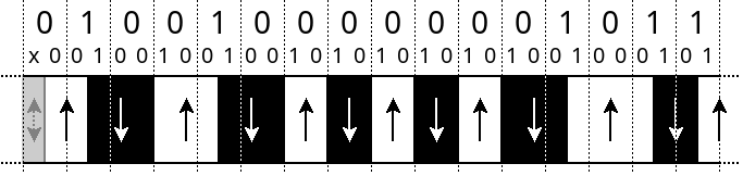
At the top you see the logical bits, those get expanded into two physical bits. Notice how every 2nd physical bit is the same as the corresponding logical bit. Then for every physical 1-bit we create a flux-reversal. Notice how these flux-reversals can now be in the middle of a logical bit. The duration between flux-reversals can be the same as the duration of single logical bit, it can be as long as 2 bits, but it can also take the duration of 1.5 bits. And important: compared to the FM-diagram, this diagram is only half as wide again.
Now that we’ve seen how single-density (SD) disks are encoded: FM. And how double-density (DD) disks are encoded: MFM. You may wonder how this is done for high-density (HD) and even extra-density (ED) disks. These are aren’t used on MSX, but just for completeness sake. Both HD and ED use the same MFM-encoding as DD disks. The difference is that the data-rate is doubled (for HD) or quadrupled (for ED) compared to DD. And this does imply that HD and ED disks are made of a material with different magnetic properties compared to SD and DD disks. On the other hand SD and DD disks do use the same magnetic material.
1.4. Other solutions (non-MSX)
We’ve seen FM- and MFM-encoding. On MSX systems these are the only two that are used on floppy disks. But other systems may use various other encodings that make different tradeoffs between efficiency, complexity, robustness, ...
One collection of such encodings that are more efficient is GCR.
2. From bit-stream to byte-stream
So far we’ve seen how to reliably store a bit-stream on a magnetic disk. However disks are circular, there’s no begin or end in a circle. This means, when reading a disk, there’s no way to know at what position in this circle the writing started. And thus, for example we don’t know how to group 8 bits into a byte. In other words, we don’t know where the byte-boundaries are located.
And strongly related: to decode an MFM stream we need to know which are the odd and which are the even physical bits. One are the useful data-bits, the other are the inserted clock-bits.
Both these problems are solved by using special marker symbols.
Revisiting MFM encoding as a transformation from an 8-bit to a 16-bit pattern
Let’s quickly revisit how a byte gets MFM-encoded:
- The 8 logical bits that make up the byte get expanded into 16 bits.
- A 1-bit always gets expanded to “01”, but a 0-bit can either expand to “00” or “10”, depending on the previous bit.
- This means that bytes that start with a 0-bit get expanded into one of two possible 16-bit patterns (depending on the last bit of the previous byte). Bytes that start with a 1-bit always get expanded to the same 16-bit pattern.
- This means that of all the 65536 possible 16-bit patterns, only 384 are obtainable by MFM-encoding.
- Most of the 65536 possible patterns are invalid, because:
- They contain two consecutive 1-bits: this cannot reliably be stored on the magnetic material.
- Or they contain more than 3 consecutive 0-bits: this may cause synchronization problems.
- If I counted correctly, there are 683 valid patterns and of these only 384 are actually used.
For example, one of these valid-but-unused patterns is “0100 0100 1000 1001” (0x4489):
- You can verify that there are no consecutive 1-bits, and at most 3 consecutive 0-bits.
- Decoding, that is: looking at the even bits, results in “1010 0001” or in hex 0xA1.
- Re-encoding this 0xA1 byte with the regular MFM-rules gives: “0100 0100 1010 1001”
More in detail:
normal A1: 0100 0100 1010 1001
special A1: 0100 0100 1000 1001Notice how the clock-bit between the 5th and 6th data-bit is 0 rather than 1.
Special MFM marker symbols
As we saw above there are 683-384=299 valid-but-unused patterns. But the special-A1-pattern from the example above has one extra property:
- Take an arbitrary sequence of input bytes, let’s say this is the arbitrary data in a 512-byte sector.
- Follow the normal MFM-encoding rules.
- Then take any 16 consecutive (physical) bits from this result. Starting at an arbitrary position, odd or even position, byte-aligned or not.
- These 16 bits will never be the same as the special-A1-pattern.
There are still other valid-but-unused patterns that also have this additional property. So in a sense this is still an arbitrary choice. But then by convention, this special-A1-pattern is given a unique meaning in MFM-disks:
- This pattern is used as a marker symbol.
- It is placed at strategic locations in the track. More on this in the next chapter about the track layout.
- It can never accidentally occur, e.g. in a sector data block, not even at sub-bit offsets.
- When this marker is found, we know where in the stream we are, and we know where the byte-boundaries are. More details later.
- And if we know the byte-boundaries, we also know which are the odd and the even (physical) bits.
FM marker symbols
In FM-encoding there is a similar mechanism with special marker patterns. But we won’t go into detail because single-density disks are anyway not used that often on MSX. If you’re interested you can find more info in the WD2793 data-sheet.
Bit order
We already established byte-boundaries: we know which groups of 8 bits form bytes. But we still need to know the bit-numbering within those bytes. Purely by convention the bits are ordered from most-significant-bit (MSB) to least-significant-bit (LSB). In other words: from bit 7 to bit 0. In fact all diagrams from chapter one were already drawn according to this convention.
3. Track layout
Quick recap: the disk rotates at 300rpm and the effective data-rate is 250k bits/s, including MFM-encoding. This results in a track-length of 6250 bytes. But note that this is the nominal track length. In practice some disk drives rotate a bit faster or slower than 300rpm (and/or the data-rate may not be exactly 250k bits/s). For example formatting a disk on my Philips NMS8250 machine gives an actual track length of around 6220 bytes (it varies a bit from disk-to-disk). Probably that’s because the drive rotates slightly too fast at 301.5rpm. But these numbers aren’t important, what is important is that there can be deviations from the ideal rotation speed. And we have to keep these deviations in mind if we want to understand the reasoning beyond the standard track-layout.
But what is this “standard track-layout”? The standard track layout for MFM disk was originally defined in 1977 for IBM System34 as follows:
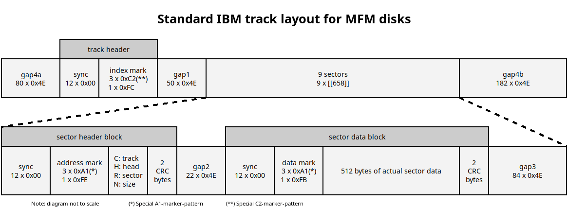
(Actually IBM system34 (1977) used 8 inch floppy disks. 3.5 inch floppy disks were only introduced in 1984. The above diagram is an adaptation of the original IBM track layout for 3.5 inch disks.)
At a high level a track consists out of:
- A track header.
- 9 sectors.
- And various gaps between the above.
A sector is further sub-divided into:
- A sector header block.
- A sector data block.
- And again gaps between these sub-structures.
Note that not all MSX machines (more specifically: the software in the MSX Disk ROM) follow this standard track layout exactly. There is some variation in the exact length of the gaps and the filler-value used in those gaps. But none of this matters for the correct functioning of the disk.
Let’s examine these structures in more detail:
3.1. Sectors
Let’s skip over the track header for now and first look at the sectors.
Why split a track into sectors?
Nominally a track can store 6250 bytes of information. But for some reason we choose to split this into 9 sectors of 512 bytes each. That’s only 4608 bytes. So we roughly loose 25% of the capacity. Why is that a good idea? Or what do we get in return?
We want to be able to modify data on disk. That is: overwrite existing data with new data. For technical reasons it’s not possible to arbitrarily modify the magnetic patterns on the disk. Instead we can only change contiguous chunks at once. Or more specifically: there must be a gap before and after the chunk we want to change. More on this later in the sections about “gaps” and about “writing a sector”.
So if we would not split a track into smaller units, and we then want to modify only a small part of that track. We would be forced to first read the whole track into memory, make the modification, and then rewrite the full track. Keep in mind that this technology was developed in the 1970s. At that time reading ~6000 bytes in memory would take a significant part of all available RAM in the machine. Think of a machine with only 16kB of RAM. In that context handling sectors of 512 bytes is already more manageable. (Some older non-MSX systems even used sectors as small as 128 bytes.)
3.1.1 Sector header block
When we want to read or write a specific sector we must be able to locate that sector in the track. That’s the purpose of the sector-header, it identifies the sector.
Sync pattern, 12 bytes of 0x00
As the name implies these are used to synchronize (or calibrate) the PLL circuit with the actual rotation speed of the disk. More in detail: match the PLL with the actual rate (=frequency) and position (=phase) of possible magnetic flux reversals.
The byte 0x00 gets MFM-encoded to the physical bit pattern ‘1010 1010 1010 1010’. This is the fastest allowed flux-reversal rate (nominally all regions 4ms long). So this is a good pattern to calibrate the PLL circuit.
The above track-layout diagram may give a false impression: it shows the gap before this sync pattern as filled with 0x4E bytes. That’s true in a freshly formatted track, and a pattern of 0x4E is good enough to keep the PLL synchronized. But these gaps don’t remain like this when the disk gets re-written often and/or in various different disk drives. More on this later. Instead we should assume that gaps can contain garbage, and then it may indeed be needed to re-calibrate the PLL with a proper sync-pattern.
Address-mark
The previous sync pattern ensured the PLL is working properly, thus we can read physical bits. However we do not yet know where the byte-boundaries are located. That’s the purpose of this ‘address mark’. It starts with 3 special-A1-symbols. In the “From bits to bytes” chapter we mentioned this symbol is used in “strategic places” in the track. This is one such place. So after we’ve seen this symbol, we’re byte-aligned and we can do proper MFM-decoding.
The 3 special-A1-symbols are followed by a 0xFE byte. This 0xFE value distinguishes an “address mark” from a “data mark” (see next sub-section about the sector data-block).
The “CHRN” bytes
After the address-mark follow 4 bytes called “C”, “H”, “R” and “N”. These are the only actual data in the sector header:
- C: This is the Cylinder number, also known as track number. Track numbers start at 0 and count up to 79 (in a normal 80-track disk).
- H: This is the Head number, also known as side number. Double sided disks have 2 sides, numbered 0 and 1.
- R: This is the Record number, also known as sector number. These start at 1 (not zero!) and count up to 9 (in a normally formatted disk).
- N: This indicates the Number of bytes in the sector. Using an exponential scale:
- 0 means: a 128 byte sector.
- 1 means: a 256 byte sector.
- 2 means: a 512 byte sector.
- 3 means: a 1024 byte sector.
- Some, but not all, disk controllers also support sizes 2048, 4096 and even 8128 bytes. But of course a 8192-byte sector does not fit in 3.5" double density disks where a full track is only 6250 bytes.
In a normally formatted track:
- All C-fields will have the same value equal to the physical track number. This information can be used to verify whether a seek-command was executed correctly. Or just to query above which track the drive head is currently located.
- All H-fields will have the same value, either 0 or 1. I can’t really think of a reason why this information is useful. Apart maybe from detecting programming mistakes? It probably exists for historic reasons.
- All N-fields will contain the value 2, indicating 512-byte sectors. (But other systems may use different sector sizes, or even a mix of different sizes within the same track.)
- The R-fields will contain the values 1 to 9. Typically the values 1-9 are encountered in natural order when the disk rotates. Though sometimes the sector numbers are interleaved, for example: 1, 6, 2, 7, 3, 8, 4, 9, 5. On older systems this might be beneficial from a performance point of view. For example: with this order, after sector 1 finished reading (and the disk keeps spinning), there’s more time before sector 2 passes under the drive head. And this extra time might be needed to prepare the CPU for reading sector 2. (On MSX this interleaved order is generally not beneficial).
2 CRC bytes
The sector header ends with 2 CRC bytes. CRC (Cyclic Redundancy Check) is an error detection mechanism. For more details on the CRC calculation see Appendix A. In this case the CRC is used to detect possible read-errors during this sector header.
The CRC-value is calculated on the full sector-header. This includes the 3 starting A1-bytes, the 0xFE byte and the 4 “C”, “H”, “R”, and “N” bytes. The resulting 16-bit value is stored in big-endian format, that is: high byte first.
Most disk controllers, when they encounter a CRC-error in the sector header, will ignore this header. If it was a transient read-error, then possibly in the next disk rotation it might be read correctly (but we only retry a few times). More details in the chapter about “reading a sector”.
3.1.2. Sector data block
The sector-data block contains the actual data for the sector identified in the preceding sector-header, typically 512 bytes.
At first sight it may seem strange to split the sector-header and sector-data into two distinct structures separated by a gap. But there’s a good reason for this, related to overwriting the sector. More on this in the chapter about “writing a sector”.
The data-block still has a finer sub-structure:
Sync pattern, 12 bytes of 0x00 (normal MFM encoding)
This serves the same purpose as in the sector header block: synchronize the PLL circuit after a gap.
Data-mark
This is similar to the address-mark in the sector header. But now the 3 A1-marker bytes are followed by 0xFB.
A normally formatted track always uses the value 0xFB as last byte in the data-mark. But disk controllers like WD2793 also recognize the value 0xF8. This is documented as a “deleted data-mark”. The WD2793 returns whether a regular or a deleted data-mark was found via the status register. On the other hand disk controllers like TC8566AF have separate read commands for regular and deleted sectors. Both controllers have separate commands to write regular or deleted sectors. I have no idea why deleted sectors are useful, they are not used in normal MSX disks. It’s probably also a leftover from an older standard.
The actual sector data
This is the actual sector data, 512 bytes long in a normally formatted track. But other sizes can be specified via the N-field of the preceding sector header.
2 CRC bytes
Directly following the sector-data are 2 CRC bytes. These are similar to the CRC in the sector-header. It includes the 4 bytes from the data-mark block, followed by the (typically 512) data bytes.
3.2. Track header
The structure of the track-header is similar to that of an address-mark or a data-mark:
- It starts with a sync-pattern (12 bytes 0x00).
- Then 3 bytes with a special-MFM symbol, but now 0xC2 instead of 0xA1. More on this in a moment.
- And it ends with one data-byte with value 0xFC.
As before: the sync-pattern synchronizes the PLL, the special-C2-symbols indicate byte-boundaries. And these are required to be able to correctly MFM-decode the 0xFC byte.
Function of the track header
We now know what the track header looks like. But what is its function? ...
... I don’t know. But I can make a guess: I think it’s a relic from an older disk standard. What I do know for sure is that this track header is not required at all for a correct functioning 3.5" floppy disk.
The next chapter will introduce the “index pulse”. In short: this is an indication somewhere along the track that can be used to count disk revolutions. From one index-pulse to the next, the disk has made one full revolution. On a 3.5" floppy disk, this index-pulse is generated by the disk/drive itself. Could it be that in other disk types there is no such physical index pulse, and instead similar functionality is obtained via some data-pattern in the track: namely this track-header?
C2 versus A1 special symbol
The track header uses special symbol C2 which has this bit-pattern “0101 0010 0010 0100” (hex: 0x5224). Decoding (=look at every 2nd bit) indeed gives the value 0xC2. Re-MFM-encoding 0xC2 results in “0101 0010 1010 0100” (hex: 0x52a4). Notice the missing clock-bit between the 4th and 5th data-bit. This is all very similar to how the special-A1-symbol is constructed. (Detail: this C2 patterns does NOT have the extra property that it cannot appear as a substring at an arbitrary offset in arbitrary but valid MFM-data.)
But why does the track header use a different special symbol? I have no idea. I think “A1 A1 A1 FC” would also have uniquely identified the track header. I guess it’s again for historic reasons, without any remaining real purpose.
3.3. Various gaps
There are 4 different gaps between the above (sub-)structures, named “gap1” through “gap4”. In a sense this is wasted space on the track. However they do play a role in the correct operation of reads and writes. We’ll visit them now, in reverse order because that’s easier to explain.
Gap4a + gap4b, between the end of the sector-data and the start of the track-header
The diagram shows “gap4a” and “gap4b” as separate gaps. But because a track is circular this is in fact a single larger gap.
Earlier we saw that the rotation rate may not be exactly 300rpm (and/or the data-rate not exactly 250k bits/s). Because of this, the length of a track may not always be exactly 6250 bytes. “gap4” serves as a buffer for this: a shorter or longer actual track-length results in a correspondingly shorter or longer “gap4”.
Gap3, between the end of one sector and the start of the next sector
When overwriting a sector, the rotation rate may not be exactly the same as the rotation rate when the track was originally formatted. Because of this the length of the newly written sector may be a bit longer or shorter than the original length that was reserved during formatting. “gap3” allows for some tolerance here.
Gap2, between the sector-header and sector-data
Rewriting data on a magnetic medium is a 2-step process:
- First the medium has to be de-magnetized, using an erase-head.
- Next it can be rewritten via the write-head, sometimes called recording-head.
The erase- and the write-head are physically separate heads (the read- and write-heads are often combined into a single head). Thus there is some physical distance between the erase- and the write-head.
This means that, once we located the position on the track where we want to write, we cannot immediately start rewriting the desired magnetic pattern. What we can do is immediately activate the erase head. But then it still takes a bit of time before the erased part of the disk has rotated under the write-head.
And this is the purpose of “gap2” between the sector header and the sector data.
Notice that overwriting a sector, does not only re-write the (512) data bytes, but the full data block, including sync-pattern, data-mark and CRC (obviously because the CRC will likely have changed). In other words: writing new data on the disk has to be done in full blocks, from one gap to the next. So we need a gap both before (gap2) and after (gap3) the sector data-block.
Gap1, between the track-header and the first sector-header
I don’t know the purpose of the track header (I’m guessing it’s only there for historic reasons). And I also don’t know why “gap1” is needed. I’m also guessing it may not strictly be needed because neither the track header nor the sector header ever get rewritten.
4. Floppy disk controller (FDC)
In principle, the previous chapters already explained all there is to know about information storage on 3.5" DD disk. In this chapter we revisit this topic from the point of view of the Floppy Disk Controller (FDC). We’ll also elaborate on some more practical aspects.
What is a Floppy disk controller and why is it needed?
In MSX computers the CPU does not directly control the disk-drive(s). Instead a “Floppy Disk Controller” (FDC) sits between them. The CPU sends commands to the FDC, and then the FDC executes these commands by sending and receiving particular (sequences of) signals to/from the disk-drive(s) it is connected to.
This differs from how the MSX controls cassette tapes. The CPU directly controls the cassette-interface without any intelligent controller in between.
Why this difference? From a distance, cassette tapes and floppy disks are similar. Both store information on a magnetic medium. Both need to encode/decode logical-bits to/from physical bits. But for cassettes this is fully done in software while for disks this is done via a dedicated hardware circuit. The software approach is more flexible: even though the default cassette encoding on MSX is FM, if you desire, it’s possible to use a different encoding. Maybe one with better error correction capabilities, or one with higher information-density. Why can’t we do the same for floppy disks? And then maybe store more than 720kB on a DD disk.
The main reason is speed: the bit-rate used on disks (250k bits/s) is a lot higher than the rate used on cassettes (without going into detail: ~5k bits/s). Also, as we learned above: 250k bits/s is the logical bit-rate, with MFM the physical bit-rate is twice as fast. So for a Z80 running at 3.57MHz that gives:
- 3579545 clock-ticks/s / (2 * 250k bits/s)
- = 7.1 clock-ticks / bit
7 clock-ticks per physical bit. That’s barely enough to execute a single (simple) Z80 instruction. Keep in mind that a full software implementation needs to include the PLL-part. That requires sampling the bit-stream (the flux-reversal-pulses) at an even higher rate (at least 3x - 4x faster). And then you still need the MFM-decoding part, the marker-symbol detection, the sector-header-interpretation, CRC-calculation, etc. So it’s easy to see that the Z80 is not fast enough. Even the R800 in MSX turbo-R machines doesn’t come close.
Off-topic: programming the FDC
MSX machines generally use a FDC from one of two main families. And the way how to program these families is totally different.
- The WD2793 family: includes WD1793, WD2793, MB8877, ...
- The TC8566AF family: includes TC8566AF, WD37C65, NEC765, ...
These FDCs are already quite old. They pre-date the 3.5" floppy disk, so some of the functions they offer are irrelevant on MSX.
The way how these FDCs (also FDCs within the same family) are accessed by the CPU can be very different between MSX manufacturers:
- Access via IO-ports or via memory?
- On which addresses? In which MSX-slot?
- Some extra stuff is not (always) controlled via the FDC. There’s also a lot of variation in how to control this:
- How to turn the drive motor on/off (to spin the disk).
- How to select the active drive. (Many FDCs can control 2, sometimes even 4, drives).
- How to read status information from the FDC, in particular the IRQ and DRQ signals used during the polling-loop (explained below). Some use positive logic, some use negative logic. Usually these two bits are read together as a byte. But the position of these bits in that byte varies.
That is all stuff we will not talk about. Instead in this article we’ll talk about:
- After a command has been send to the FDC, what are the sub-tasks that the FDC will perform.
- And then in particular: how does this relate to the information (the magnetic patterns) that is stored on the disk.
More concretely we’ll look at the commands:
- Read a sector.
- Write a sector.
- Format a track.
Prior requirements
Before the read-/write-sector or format-track commands can be executed, there are some prior requirements:
- The correct drive must be selected (in case one FDC controls multiple drives).
- The disk must already be spinning (the drive motor must be turned on).
- The correct side of the disk must be selected (for double-sided disks).
- The drive head must be located above the correct physical track. (Typically accomplished via FDC seek commands.)
How to do this is also outside the scope of this article.
Index pulse
Before delving into the details of the FDC commands, there’s one more hardware aspect we need to know about: the index pulse.
Once per rotation, the disk-drive sends a pulse to the FDC. Via this pulse the FDC can count how many rotations the disk has made. So the index pulse marks one specific (rotational) position of the disk. You could interpret this as the start (and/or as the end) of the track.
And this is the only feedback the FDC receives about the position of the disk. Apart from the index-pulse, the FDC has no idea how far along the disk has rotated (what the current rotation angle is).
4.1. In detail: reading a sector
The disk is already rotating, the correct drive/side/track has been selected. A sector-read command for a specific sector-number has just been given. What happens next?
From a high level:
- We’ll first locate the sector (via the sector-header).
- Then we’ll locate the following sector-data-block.
- We transfer the data from this block to the CPU.
- And at the end we report a possible read-error (detected via a 16-bit CRC).
Locate the sector
At the moment the read-sector command is started, the FDC has no idea where that specific sector is located on the disk in relation to the current position of the disk (at what rotation-angle). In other words: we start reading at a random position in the track and have no idea how far the disk must turn to read the requested sector.
Also there’s no fixed order of the sectors in the track. Typically the sectors are numbered 1-9, and also appear in that order. But in some cases sectors can e.g. be interleaved (or copy-protected disks may use other sector numbers than 1-9). That means the FDC cannot make any assumption about were a specific sector is supposed to be in the track. The only the thing the FDC can do is read all sector headers until a match is found.
In the best case the correct sector-header will be found soon, in the worst case it can take up-to a full disk-revolution (at 300rpm a full revolution takes 0.2 seconds). It can also happen that the requested sector is not found at all during one revolution. We don’t want to keep searching forever, so what FDCs do is count the number of ‘index pulses’: if the sector is not found within 3 or 5 index pulses, then stop the command and report a failure. Searching for more than 1 revolution allows for some retries in case of (transient) read-errors.
Read the sector header
So the FDC tries to locate the matching sector-header. How does that work exactly? Basically we look for an address-mark, and then compare the following “CHRN” bytes with the desired values. But it’s a bit more complicated than that:
- Reading data means measure the durations between flux-reversals and interpret these as MFM patterns.
- Though when we just start reading, the PLL may not yet be synchronized, and then we don’t even know where the bits are.
- Normally the PLL will be synchronized pretty quickly. At least when there are valid MFM-patterns passing under the read-head. Unfortunately this may not always be the case. In a freshly formatted track, the various gaps contain clean filler-bytes. But as we’ll see below in the section about “writing a sector”, these gaps can accumulate garbage magnetic patterns. So to ensure the PLL will always correctly synchronize there is a sync-block after every gap.
- Similarly when we just started to read (and possibly again after every gap containing garbage) we do not yet know where byte-boundaries are located. As explained in the “From bit-stream to byte-stream” chapter, this is done via the special-A1-symbol. More in detail: the FDC has a 16-bit shift-register. Every newly read physical bit gets pushed into this register and an old bit drops out. When this register contains the value “0100 0100 1000 1001” (0x4489) we found our special-A1-symbol, and then we can synchronize the byte-boundaries.
So after a while both the PLL and byte-boundaries are synchronized. At that point the MFM-decoder is fully operational, and we can start to actually interpret the data in the track. We still need to locate the correct sector-header.
- The first sub-step is to look for an address-mark. This can be recognized by 3 special-A1-symbols followed by a (normal) 0xFE byte.
- Once the address-mark is found, we read the next 4 bytes. These are respectively the C, H, R and N fields in the sector-header.
- We compare the value of the “R” field (= record = sector) with the to-be-located sector number. If it’s different, we continue searching for the next sector-header. If it’s the same, then continue with the next step.
- After the C,H,R,N bytes follow 2 CRC bytes. These are compared with the current running CRC value, more on this in a moment. If there’s a mismatch, then this sector-header is ignored and we continue to search for the next sector-header. If the CRC did match we’ll search for the sector-data-block.
But first more about the running CRC value:
- On each byte that was read, the FDC also updates an internal 16-bit CRC with the value of that byte. See appendix A for details on this calculation.
- When a special-A1-symbol is read, the internal CRC value is reset to 0xFFFF(*).
- This means that the CRC-value stored in the sector-header is calculated on the full sector-header, including the 4 bytes from the address-mark. But no prior bytes from e.g. the sync-block or the gaps.
(*) Maybe the CRC is only reset to 0xFFFF on the first in a sequence of consecutive A1-symbols, or maybe each A1-symbol resets the value to something else than 0xFFFF. (Impossible to know, and maybe different FDCs handle this in a different way). In any case the effect is as-if the CRC is calculated on the 8 bytes: 0xA1 0xA1 0xA1 0xFE [C] [H] [R] [N].
Locate the sector-data-block
After a matching sector-header was found, we search for the following sector-data-block. This is done by looking for a sequence of 3x special-A1-symbols followed by a 0xFB byte, this is called the “data-mark”. The data-mark must occur within 43 bytes after the sector-header. If not found within that window, we restart searching for another matching sector-header.
Note that prior to the data-mark is again a sync-block (to train the PLL) and the data-mark contains special A1-symbols to synchronize the MFM-decoder on byte-boundaries. You may think that’s unnecessary because we already were fully synchronized after reading the sector-header. That’s indeed true in a freshly formatted track. But it doesn’t remain true when this sector has been overwritten. More on this in the section about “writing a sector”.
Detail: the normal data-mark contains 0xFB as the last-byte. But the value 0xF8 is also recognized. This is called a deleted data-mark. I don’t know what the use case for this is. It’s probably a leftover from an older standard. The WD2793 family of FDCs reports such a deleted sector via a status bit after the read-sector command finishes. The TC8566AF family has separate read-commands for both sector types.
Transfer data to the CPU
After the data-mark was found, the actual sector-data is read. In a normally formatted track the length of this data-block will be 512 bytes, but the FDC gets the actual length from the N-field in the prior sector-header.
The FDC reads and decodes each data-byte and makes it available for the CPU. More in detail: the CPU should poll the FDC to check if a new data-byte is available, then quickly read it from the FDC and store it in RAM. The FDC only has a buffer for a single byte. This means the CPU-polling-loop should run fast enough to keep up with the FDC. Because the disk won’t stop rotating when the CPU is too slow. If I counted correctly: at 3.57MHz, the Z80 has ~114 cycles to process each byte.
Similar as for the sector-header, the FDC keeps a running CRC value. When all (512) bytes in the data-block have been read, the FDC reads 2 additional CRC bytes, and compares those with the running CRC value. And similar as for the header: the values 0xA1 0xA1 0xA1 0xFB from the data-mark are included in the CRC-calculation.
One difference between sector-header and sector-data is that, on a CRC-error, there’s no automatic retry. Instead the command reports a mismatch as a CRC-error. But in the mean-time all data-bytes have already been transferred.
Detail: right after the data-mark has been read, during reading of the actual sector data, the special-A1-symbol detector (the 16-bit shift-register) is turned off. In other words during the data-block we will not re-synchronize byte-boundaries. Theoretically such special-A1-symbols cannot occur during the data-block (not even at arbitrary sub-bit offsets). But maybe this is more robust in case of read-errors?
4.2. In detail: writing a sector
The start of a write-sector command is identical to the start of a read-sector command. We first have to locate the sector in the track. This is done by locating a matching sector-header. See the previous section “reading a sector” for details on this step.
After the sector-header has been found, the write-sector command fully overwrites the data-block. This works as follows:
- After the sector-header, we wait for the duration of 22 bytes (the standard gap-length between sector-header and sector-data-block).
- Next we write a new sync-pattern: 12 bytes of 0x00.
- Followed by a data-mark: 3x special-A1-symbol and a 0xFB byte (or 0xF8 for a deleted-sector).
- Then the (usually 512) actual data-bytes are written. Similar as for reading: the CPU must provide these bytes fast enough, using a tight polling loop.
- After the last data byte has been written, the FDC automatically appends two CRC bytes. The CRC-calculation is identical as for the read-sector command.
- And finally one 0xFE byte is written. I’m not exactly sure what the purpose of this byte is. E.g. it’s not part of the standard IBM track layout.
Note: the track was formatted with a certain gap-length (gap2) between the end of the sector-header and the start of the data-block. This may have been a different length as the standard IBM gap2-length. However after re-writing the sector, this gap is restored to the standard length of 22 bytes. In other words: this part of the formatting is not preserved.
Remember that the nominal rotation rate is 300rpm, but the actual drive may have a slightly different rate. In particular the rotation rate when the track was formatted may be different from the rate when the sector is overwritten. During reading we can synchronize on the prior recording speed (via the PLL), but this is not possible during writing. This is because writing is a two-step process: first we demagnetize the to-be-overwritten part of the disk, then we write a new magnetic pattern. So during the write-process there really is no magnetic pattern left on the disk for the PLL to synchronize on.
Because of this possible difference in rotation rate, after a re-write, “gap2” and “gap3” may have a different length. And the new length may not be a multiple of a full byte anymore. In other words: some filler bytes in the gap may have been partly overwritten. And the new magnetic pattern on the transition may not even satisfy all MFM-encoding-constraints anymore (no two 1-bits directly after each other, and at most three 0-bits between two 1-bits).
Also demagnetizing (via the erase-head) requires a stronger magnetic field than writing new data (via the write-head). Thus erasing is a more blunt operation, while writing can be more precise. The erase- and the write head have some distance between them, it takes a little bit of time before the erased part of the disk has rotated under the write-head. So activating the erase-head should happen a little bit before writing can happen (I’m not exactly sure how the FDCs handle this). But this means that erasing and re-writing may not be perfectly aligned on the disk. So there can be small parts on the disk that were erased but not-rewritten. Or there can be small parts that were not erased but are rewritten. In other words: it’s not possible to very precisely change the magnetic patterns in one region, while leaving the parts directly in front and directly after perfectly in tact.
The previous two paragraphs both explain why the gaps around the sector-data-block are needed. And why, after a rewrite, these gaps can contain garbage. Rather than clean filler-bytes, as in freshly formatted track. In summary: we always need to re-write whole blocks, from one gap to the next. And these gaps should be considered to contain (some) garbage after a re-write.
4.3. In detail: formatting a track
In the data-sheets this is sometimes called “writing a track” or sometimes “formatting a track”. From a FDC point of view, formatting a full track is actually a lot simpler compared to reading/write a sector. Basically we need to:
- Wait for the “index pulse”.
- Start writing the track-layout.
- Continue doing this till the next “index pulse”. In other words: write for one full disk rotation.
But of course the 2nd point “write the track-layout” still hides a lot of complexity inside. We’ll address it in a moment.
Remember that the rotation-rate is not exact, so this command will not write exactly 6250 bytes. It may not even be an integer multiple of a byte. Normally this variation in rotation speed is small enough to only affect “gap4”, that is the gap after the last sector and before the track-header.
Now about point 2: “writing the track layout”. This part is handled totally different in the TC8566AF and the WD2793 family of FDCs.
Format-track command on the TC8566AF family
The TC8566AF format command only takes a few parameters and then more or less independently writes the track. These parameters are:
- The sector size. A single size parameter implies that all sectors in the track will have the same size.
- The number of sectors in the track.
- The length of “gap3”, that is the gap between the end of a sector and the start of the next one.
- The value for the data-byte. The data-blocks of all sectors are filled with this single byte.
- And per sector: the value for the “C”, “H”, “R” and “N” fields in the sector-header.
So this command only gives a little bit of freedom. In other words: it can only produce tracks that are fairly close to the standard IBM track layout. For normal use this is perfect: it makes this command easy to use. But it doesn’t allow for intentional deviations from the standard track layout (e.g. to create some kind of copy-protection).
Write-track command on the WD2793 family
In contrast, the “write track” command on the WD2793 gives almost full control to the CPU to write the track-layout. That is: every byte that’s written to the track must be send by the CPU (in a polling-loop, similar as for the write-sector command).
However there are some complications:
- Formatting a track also requires to write the 2 special A1 and C2 symbols (see section on “MFM marker symbols”).
- So the CPU cannot simply send the bytes 0xA1 and 0xC2 because those would be written as normally MFM encoded bytes.
- The solution is to reserve 2 values: 0xF5 and 0xF6. These will respectively write a special A1- or C2-symbol.
- But the disadvantage is then of course that the write track command can no longer write normal 0xF5 or 0xF6 bytes.
- Usually that’s fine. A standard track doesn’t contain those values. Except:
- In the sector data-blocks. This means that, in general, “write track” cannot both format the track and simultaneous fill the sector blocks with the correct values.
- The 2 CRC-bytes might have the value 0xF5 or 0xF6. To solve this the WD2793 reserves a 3rd value: 0xF7. When the CPU sends this byte, the FDC will write 2 CRC bytes instead of a normal 0xF7 MFM value. The CRC is calculated in much the same way as for the write-sector command. As a bonus this frees to CPU from the non-trivial CRC-computation.
So this command gives a lot of control over the track-layout. If the goal is to create a standard track layout, then this only adds a lot of complexity. On the other hand if you intentionally want to create non-standard tracks (e.g. to create some copy-protection), this opens some possibilities.
4.4. Other FDC commands
This article is not about FDC programming. I only want to mention some other commands that are commonly available on FDCs. But for details you’ll have to read the FDC data sheets.
- Seek command(s): to move the drive head to a different physical track.
- A diagnostic command to read the content of sector-headers. (At least on WD2793) this can be used to detect/read sector-headers which have a CRC error. Or read a sector-header without a corresponding sector-data-block. (Because the regular read-sector command will skip both such headers).
- A diagnostic command to read the full content of the track. This only returns bytes in the range 0-255, so for example it doesn’t give enough information to distinguish a normal-A1 from a special-A1-symbol. This command is not always reliable (I mean it returns unreliable data) when there’s garbage in the various gaps. Or it returns bogus data before a special-A1-symbol has been seen (e.g. when the command was just started).
Appendix A: CRC calculation for “CRC-16-CCITT”
CRC is short for Cyclic Redundancy Check. It’s a family of codes that can be used to detect errors. But they cannot correct errors. For much more details on CRC in general, check this wikipedia article.
In this appendix we’ll specifically talk about the CRC-16-CCITT version. On floppy disks this CRC is used to detect read errors in the sector-header and sector-data blocks. It’s a 16-bit CRC with start value 0xFFFF and polynomial: x16+x12+x5+1 (see wikipedia for what this means). Here we’ll only show how to calculate this CRC:
Algorithm: incrementally calculate the CRC, byte-per-byte:
    // Update the current running CRC-value with a new data-byte.
    // Inputs:
    //   crc: the current 16-bit CRC value.
    //   value: the new input-value (8-bits).
    // Output:
    //   The updated CRC-value.
    uint16_t update_crc(uint16_t crc, uint8_t value)
    {
        for (int i = 8; i < 16; ++i) {
            crc = (crc << 1) ^ ((((crc ^ (value << i)) & 0x8000) ? 0x1021 : 0));
        }
        return crc;
    }
Example usage: calculate the CRC for a whole buffer:
    uint16_t calculate_crc(uint8_t* buffer, size_t length)
    {
        uint16_t crc = 0xffff; // start value
        for (size_t i = 0; i < length; ++i) {
            crc = update_crc(crc, buffer[i]);
        }
        return crc;
    }
This is just an example implementation. Depending on the context there might be better implementations with different tradeoffs between speed and memory usage. E.g. by using a lookup table.
Wouter Vermaelen, 2022/05/16